This is the first post in my Georgia Tech series, which is where I will post the blog-like assignments that I had to write as a part of my coursework. Much of the technical work of the original writeup has been removed to better cater to a broader audience.

Introduction

This post was originally written in December of 2021 as a part of my final report for a Data Mining and Statistical Learning course at Georgia Tech. Since it was written a 72-page report on April 27th, 2022 was released that documented the results of a two-year investigation by the Minnesota Department of Human Rights. In summary, it found:

there is probable cause that the City and MPD [Minneapolis Police Department] engage in a pattern or practice of race discrimination in violation of the Minnesota Human Rights Act. ¹

with findings that:

MPD uses covert social media to target Black leaders, Black organizations, and elected officials without a public safety objective ²

and most shockingly:

This analysis shows that MPD officers searched 16.1% of Black individuals or their vehicles during a traffic stop and searched 8.8% of white individuals or their vehicles. Even when comparing only similar traffic stops, MPD officers searched Black individuals or their vehicles during a traffic stop almost twice as often compared to white individuals and their vehicles ³

While search rates are close to 2X for black individuals as white, I wanted to dig deeper and see if these disparities existed when controlling for other factors. At first look, there are strong disparities between treatment across races during traffic stops but what about income, time of day, and income of the neighborhood? The more I can control for these in my analysis, the sturdier any claims made will be.

Note: You may notice that my search rates are higher than the investigation found. I don’t currently know the source of the difference, but it may be a difference in methods, data source, or both. My current theory is that a null value in the personSearch and vehicleSearch columns was interpreted as no search occurring by the MDOH. I decided to ignore these values instead. I contacted MDOH and If this theory can be confirmed I will change my analysis and add an edit here.

Data Sources

Open Minneapolis Police Stop Data

The first of two data sources used in this analysis is the Police Stop data set from Open Minneapolis. Open Minneapolis is a website run by the city of Minneapolis that:

seeks to provide increased access to public spatial geographic information systems (GIS) and non-spatial data that is regularly requested by private citizens and businesses ⁴

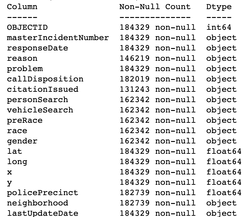
The website has data sets ranging from Public Safety, Administrative Boundaries, Planning, and even Scooter data. The Police Stop data set has 185k records of police stops from November 2016 to November 2021. Within the data set there is information on the following:

• Date of the stop
• Whether the vehicle was searched
• Whether the person was searched
• Race and gender of the person stopped
• Latitude and longitude of where the stop occurred
• Precinct that the stop occurred within
• Neighborhood of the stop

Census Income by Census Tract

The other data set I used in this analysis is a simple table that contains the income of each Census tract in Minneapolis, and its income per capita for those over 25. A Census tract is the smallest aggregation level for the United States Census. This small geographical area allows for granular reporting around any question the census asks and is much more granular than the county, city, or even neighborhood level statistics (at least in Minneapolis).

Why Use Income for Those Over 25?

The reason for using income over age 25 vs no age restriction has to do with a large concentration of university students within the Dinkytown neighborhood of Minneapolis. If I were to have just used per capita income without age considered, it would make it seem that the neighborhood is one of the most impoverished and lacking resources. This is because many college students likely have low-wage, low-hours jobs or none at all. Instead, their spending and tuition are likely supported by parents and loans. Due to this, using income over 25 likely reflects the incomes of those who have dependents and the socioeconomic status of the neighborhood.

Analysis and Results

EDA

Before machine learning, I observed possible relationships with a search and other variables in the data set.

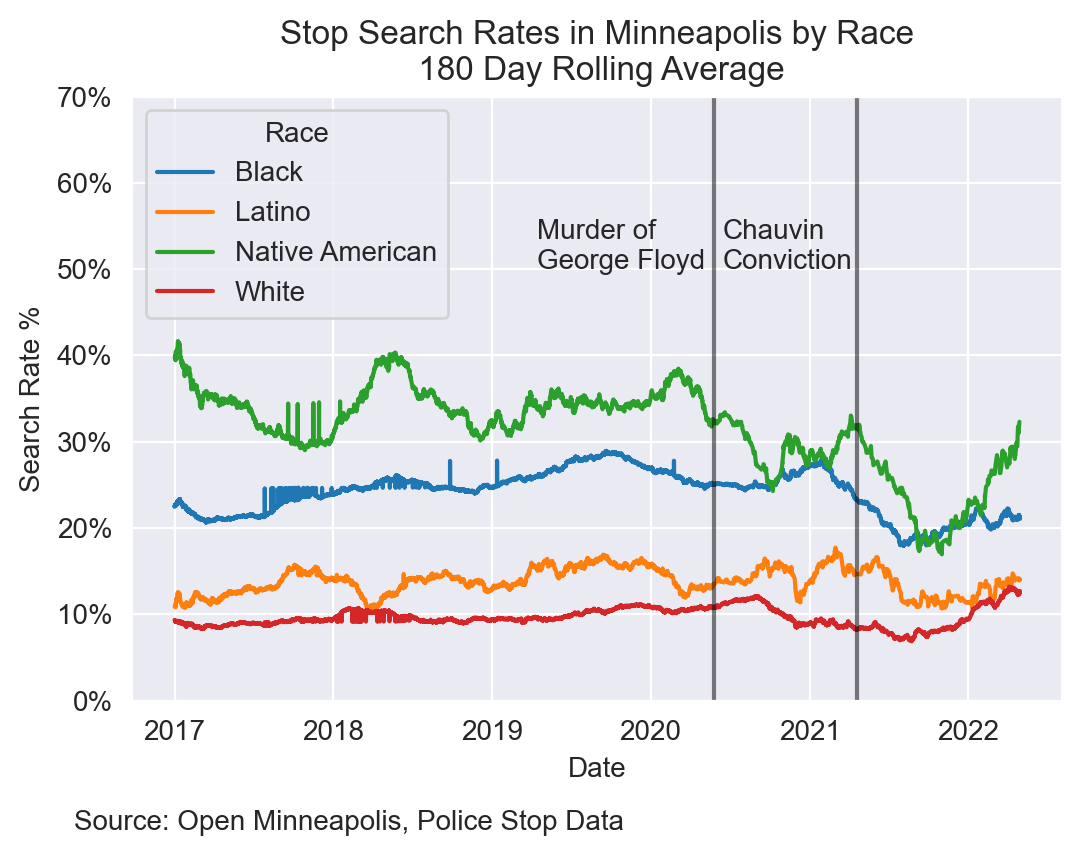
Race

First, I wanted to observe the relationship between search rates and race over time. The gap between those who are White and those who are Black or Native American has been rather steady from 2017 through the beginning of 2020. After the murder of George Floyd and especially the Chauvin Conviction, search rates rapidly decreased for those who are Native American or Black. These events seem to have little or no effect on those who are Latino or White.

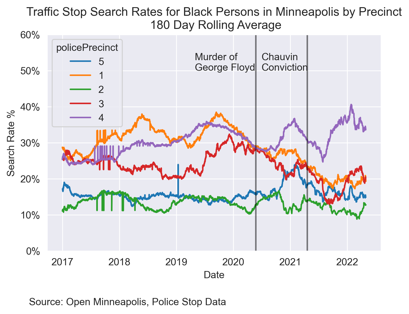
Precinct

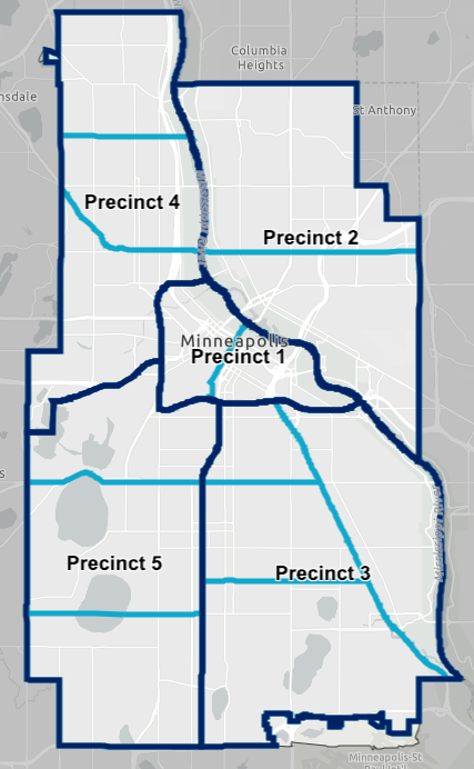
While race looks to be a component in understanding search rates, it is also worthwhile to understand the differences within the police districts in Minneapolis, since they may have different methods of policing.

Below is a map of the five different precincts within Minneapolis and their rates of search of Black persons by Date. There were differences in search rates by precinct before the two events on the graph, but all precincts’ search rates stayed more or less the same. The one exception was Precinct 4 in Northwest Minneapolis. After the two events, Precinct 4 became the precinct with the highest search rate, at around 37.5%.

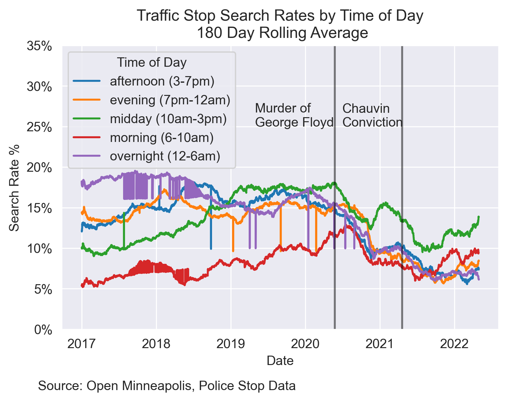
Time of Day

Additionally, a lack of daylight or previous patterns of crime throughout the day may cause police to have more or less suspicion at different times.

Before 2019, the “later” in the day, the more likely someone stopped was to be searched. Since 2019 there are close to no gaps between different times of the day.

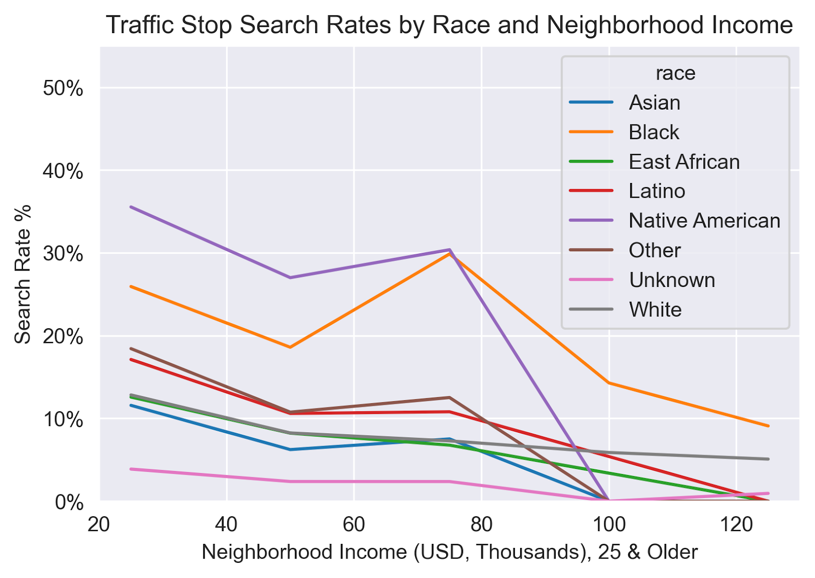
Race & Income

Lastly, the cross-sectional relationship of race, income, and date was explored. For all races as income increased in the local Census Tract of the stop, search rates decreased in a somewhat linear fashion.

Machine Learning Results & Metrics Interpretation

The original audience of my Georgia Tech Peers had an understanding of what ROC AUC was. To learn more about this useful and common machine learning metrics, see here. If you aren’t interested in the technical aspects, skip to here

Logistic Regression

First, a Logistic Regression was run, and the model performed similarly to randomly guessing if someone was pulled over or not, given its ROC AUC of 56%.

Random Forest

Conversely, the Random Forest with no parameter tuning had a ROC AUC of 69%. This means that the Random Forest is much better than guessing at random when it comes to discerning whether someone will be searched or not but still far from perfect.

AutoML - XGBoost

Lastly, the AutoML algorithm that selected a tuned XGBoost model had an AUC of 78%! This means that XGBoost was the best of the three models at discerning between searches and non-searches during police stops. As shown in the ROC curve below, at a certain threshold the model was able to correctly classify >80% of the stops that resulted in searches while only misclassifying 40% of non-searches as searches.

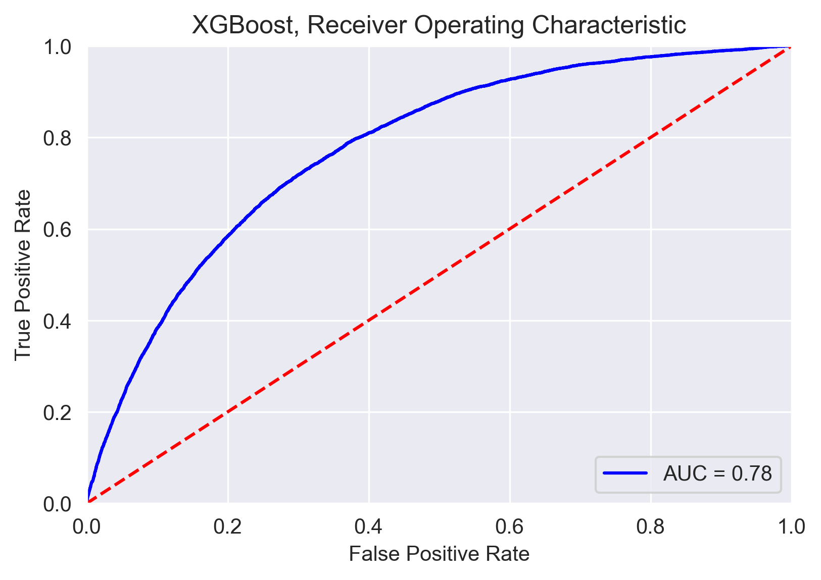
The fact that this was the most powerful model is unsurprising since I used an algorithm that intelligently looped through different models and parameter spaces.

Let’s look at what features were the most important in our most performant model, XGBoost.

XGBoost Shap Values

So what variables are most important and helpful in discerning whether a search will be conducted during a police stop? To better understand the answer to this question, I will first need to understand what “Shap Values” are.

Since XGBoost and any other tree-based models are nonlinear, I am unable to make interpretations such as “those of the black race are 3X as likely to be searched in a stop, holding all other variables equal”.

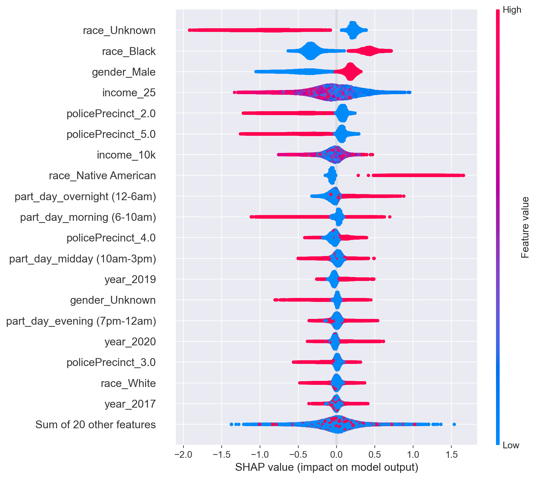
This is where shap scores come in. Each dot (there are 150k+ of them) in each row is the log odds or $e^{(log\ odds)} = odds$, which I will discuss later) of the variable for that stop. As for the color of the dot, red denotes if the value is high and blue is low. For example, rows with a race_Black of 1 (meaning the person stopped was black) have higher shap values

So What Do the Shap Scores Tell Us?

If I picked a dot that was 1.0 for race_black, this means that for this specific stop (a stop in a certain precinct, time of day, etc) that being black made the person (or their vehicle) e^1 times (2.72X) as likely to be searched.

This graph allows us to see what variables influence the model the most and in what way. From the graph it is clear that the race of the individual, their gender, what time it is, and the income of the neighborhood they are in are very influential when it comes to being searched.

A couple of nonlinear effects stand out. Many variables have a clear relationship with leading to a greater/less chance of being pulled over. part_day_overnight (time of day = overnight) and income_25 (income of those over 25) especially have more complex relationships with being searched or not since red and value values don’t necessarily denote higher or lower shap values.

In a future analysis exploring what other variables cause income and time of day to either have a positive or negative influence would be of interest. It could be the case that certain races are more likely to be searched at night, while others are not affected by the time of day.

Conclusions

Overall, I am pleased that I was able to develop a model that was rather predictive for this assignment, but what that means for the outside world is muddied. If a few simple features can easily predict whether or not someone will be searched, it may be the case that there is unfair bias against the features that I saw lead to more searches such as being Black or Native American, Male, and in Precinct 4.

That being said, for the model to be properly interpreted as a sign of police bias against certain groups and situations, I would likely need to control for more aspects of the stop. Aspects such as the criminal record for the stop and reason for suspicion/search (was it subjective or for something more objective?) would give more insight into if there was a justified reason for a search or not.

Additionally, to improve the model’s performance, the racial composition of the neighborhood the stop was in would help understand the effect of being pulled over in a primarily different neighborhood or the same race as your own.

Neighborhood racial composition and many other additional features would be interesting to explore, but I’m pleased with the performance of the models. I plan on sharing this work with my city’s council to help address the question of police bias in Minneapolis.

Discuss on HN